The SSP model predictions
By default model predictions
Since the formats in which SSP model predictions are provided by the different authors are also very different, rmodel assumes that the input data is available in a specific format, specially devised for this program.
The directory where the auxiliary files were installed (by default
/usr/local/share/rmodel) contains a subdirectory called models, which
includes the by default SSP model predictions available for the interpolation.
For each model, at least two files must be present. For example, considering
the Bruzual_Charlot_2003 models, there are two files called:
model_bc03.def
model_bc03.dat
The file model_bc03.def defines the number of free parameters (4 in this
case, namely age, measurement type, metallicity and IMF). For each of these
parameters, the file contains all the possible values (one per line). An
exclamation mark (!) at the beginning of a line indicates that the
corresponding value will be skipped. These exclamation marks can be changed at
any time before the execution of rmodel. In this way the user can freely
define and modify the grid that will be used in the interpolations.
Finally, the file model_bc03.def contains the list of line-strength indices
predicted by the models. The names of the indices must match the syntax
employed in the file definitions/myindex.rmodel (located in the
installation directory) and which contains the precise index definitions,
including the bandpass limits. These numbers are used by the program to compute
the index-dependent error coefficients “c” (see Equation 3 in
Cardiel_etal_2003). Some of the indices, like [MgFe], have a special syntax,
since they are computed as a (mathematical) combination of other line-strength
indices.
The file model_bc03.dat contains the model predictions, and should not be
modified. This file is an ASCII table listing the different line-strength index
predictions in each column, with the SSP parameters varying sequentially in the
order in which they appear in the file model_bc03.def.
In the current version of the program, the following SSP model predictions have been included:
Bruzual & Charlot (version 2001)
Vazdekis_etal_2003, updated with modifications from Vazdekis (2008; see also Vazdekis_etal_2007)
Using different model predictions
It is possible to use model predictions different from those included by default in rmodel. In order to use this option, the user must generate two files in the working directory:
model_user.def
model_user.dat
The formats of these files are the same previously explained for the files
model_bc03.def and model_bc03.dat, so it is advisable to have a look to
those files in order to understand the explanation that follows.
model_user.def: the first line of this file contains a description of the models. Here you can use any text you want (preserving the “#” symbol as the first character of the line). The second line is just a separator. The third line contains the number of parameters (e.g. age, metallicity, IMF, etc.) for which the models provide predictions. After that, the file must contain the description of all the values available for those parameters. As previously explained, an exclamation mark (!) at the beginning of a line indicates that the corresponding value will be skipped by rmodel (in this way the user can, in principle, modify the model grid displayed and employed by rmodel). Finally, the file must contain the list of line-strength indices predicted by the models, using the same syntax employed in the filemyindex.rmodel(located under the definitions subdirectory of the source directory) .model_user.dat: this file is an ASCII table containing the actual model predictions. The first columns contain (in ascending order!) the values of the model parameters (e.g. age, metallicity, IMF, etc.), following the same order used in the filemodel_user.def. It is very important to note that this file must contain the predictions for all the possible values of the parameters, including those signaled with an exclamation mark (!) in model_user.def. Thus, the first column contains the first parameter, the second column the second parameter, and so on. These parameters must be listed sequentially, with all the values of the first parameter changing before modifying the second parameter, etc. The rest of the columns must contain the line-strength values in the same order listed in the filemodel_user.def.
In addition, if the new models predict line-strength indices that are not
included in the file myindex.rmodel, the new indices should be defined in
that file.
IMPORTANT: After modifying the file myindex.rmodel, it is necessary to
reinstall the package in order to guarantee that the modified version of
myindex.rmodel is placed in the correct installation directory. This
implies to repeat some of the installation commands previously described:
$ make clean
$ make
$ sudo make install
Modifigying myindex.rmodel
Note that, due to historical reasons, the names of the indices (first column) should not exceed 8 characters long. The second column is an integer number that allows the identification of the type of line-strength feature. The code employed in this column is the following:
index code |
type of index |
examples |
|---|---|---|
1 |
molecular |
CN1, CN2, Mg1, Mg2, TiO1, TiO2,… |
2 |
atomic |
Ca4227, G4300, Fe4668, Hbeta, Fe5270, Fe5335,… |
3 |
D4000-like |
D4000 |
4 |
B4000-like |
B4000 |
5 |
color-like |
infrared CO_KH |
10 |
emission line |
OII3727e |
[11..99] |
generic discontinuity |
D_CO,… |
[101..9999] |
generic index |
CaT, PaT, CaT*,… |
[-99..-2] |
slope index |
sTiO |
Although the file myindex.rmodel can be easily edited and modified by any program user to include new index definitions (of the type previously described), it is important to keep the file format in order to guarantee that rmodel works properly.
An example of some of the definitions that can be found in the file
myindex.rmodel is the following (the list shown here is not complete!):
Index    code    blue bandpass      central bandpass      red bandpass     >              source
======== ====  ==================  ==================  ==================    ======================================
CN1         1  4080.125  4117.625  4142.125  4177.125  4244.125  4284.125  > Lick
HdA         2  4041.600  4079.750  4083.500  4122.250  4128.500  4161.000  > Hdelta A (Worthey & Ottaviani 1997)
D4000       3  3750.000  3950.000  4050.000  4250.000     0.000     0.000  > 4000 break (Bruzual 1983)
B4000       4  3750.000  3950.000  4050.000  4250.000     0.000     0.000  > 4000 break (Gorgas et al. 1999)
CO_KH       5  22872.83  22925.26  22930.52  22983.22  00000.00  00000.00  > Kleinmann & Hall (1986)
D_CO       12  > generic CO discontinuity (Marmol-Queralto et al. 2008)
               22880.00  23010.00
               22460.00  22550.00
               22710.00  22770.00
CaT_star  506  > CaT* index from Cenarro et al.(2001) (Paschen-corrected near-IR Ca triplet)
               8474.000  8484.000
               8563.000  8577.000
               8619.000  8642.000
               8700.000  8725.000
               8776.000  8792.000
               8461.000  8474.000  -0.93
               8484.000  8513.000  1.0
               8522.000  8562.000  1.0
               8577.000  8619.000  -0.93
               8642.000  8682.000  1.0
               8730.000  8772.000  -0.93
The two classical line-strength indices typically employed in the literature, molecular (index code = 1) and atomic (index code = 2) are defined with the help of 3 bandpasses, which appear in the following columns of each index entry of the file myindex.rmodel. Among the most common sets of molecular and atomic indices, one of the most widely used is the Lick/IDS system (see e.g. Trager_etal_1998 and references therein).
Two types of simple discontinuity indices are exemplified by the D4000 (index code = 3) and the B4000 (index code =4); see e.g. Gorgas_etal_1999. In both cases, the line-strength index is defined as the ratio between the integrated flux in two nearby bandpasses. The difference between the D4000 and the B4000 like indices is the way in which the flux in each bandpass is integrated. In D4000-like indices, and due to historical reasons (e.g. Bruzual_1983), the total flux in each bandpass is computed as the integral
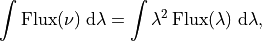
extended over the wavelength range of the considered bandpass.
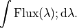
In the other hand, the total flux in each band of the B4000-like indices are obtained through the, more intuitive, integral of
The color-like index (index code = 5), defined with two bandpasses as
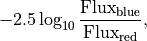
is exemplified by the CO index at 2.1 microns CO_KH (e.g. Kleinmann_Hall_1986).
Emission line features (index code=10) are measured by defining an arbitrary number of continuum and feature regions. The format to define this kind of index in the file
myindex.rmodelconsists in providing the total number of regions in the second line, and the wavelength limits of each band followed by a factor in the subsequent lines. When this factor is equal to 0.0, the region is used to compute the continuum, whereas a factor equal to 1.0 indicates emission-line region (see e.g. definition of OII3727e). All the continuum regions are fitted using a straight line fit.Generic discontinuities (index code:
 ) can be used
to define discontinuities with a variable number of wavelength regions at
both sides of the discontinuity. The integer value of
) can be used
to define discontinuities with a variable number of wavelength regions at
both sides of the discontinuity. The integer value of  in
the second column of the file
in
the second column of the file myindex.rmodelis computed as , where
 and
and  are, respectively, the number of
continuum and absorption spectral bandpasses at both sides of the
discontinuity. For this kind of index, the wavelengths which define each
bandpass are given in different rows in the file myindex.rmodel For
illustration, see Marmol-Queralto_etal_2008 for a detailed definition of the
D_C0 index.
are, respectively, the number of
continuum and absorption spectral bandpasses at both sides of the
discontinuity. For this kind of index, the wavelengths which define each
bandpass are given in different rows in the file myindex.rmodel For
illustration, see Marmol-Queralto_etal_2008 for a detailed definition of the
D_C0 index.The slope indices are derived through the fit of a straight line to an arbitrary number of bandpasses (ranging from 2 to 99). The integer value of
in myindex.rmodelindicates the number of bandpasses with a negative sign. The derived indices correspond to the ratio of two fluxes, evaluated at the central wavelength of the reddest and bluest bandpasses.